Molecular Orbital (MO) projected Density-of-States - MolPDOS
Basics
This mode allows to generate projections and pDOS plots with respect to any molecular orbital (MO). To run it one has to add following keyword to <seed>.param
%BLOCK DEVEL_CODE
  MolPDOS
%ENDBLOCK DEVEL_CODE
The projection data is produced by CASTEP after the SCF task and is written to files called <seed>.molpdos_state_<#>_<#>, where the two numbers correspond to the number and the spin of the specified reference orbital from the reference checkfile.
At the end of the <seed>.castep file the projection is commented in the following way:
Successfully read .deltascf file!
              Calculating MolPDOS weights
+-------------------INPUT PARAMETERS-------------------+
Taking band from model    gasphase
MolPDOS state               1
MolPDOS band  nr.           4
MolPDOS band has spin      1
MolPDOS state               2
MolPDOS band  nr.           5
MolPDOS band has spin      1
MolPDOS state               3
MolPDOS band  nr.           6
MolPDOS band has spin      1
MolPDOS state               4
MolPDOS band  nr.           4
MolPDOS band has spin      2
MolPDOS state               5
MolPDOS band  nr.           5
MolPDOS band has spin      2
MolPDOS state               6
MolPDOS band  nr.           6
MolPDOS band has spin      2
|DeltaSCF| Reading projection data from model file gs.check
Writing file   no.molpdos_state_4_1
Writing file   no.molpdos_state_5_1
Writing file   no.molpdos_state_6_1
Writing file   no.molpdos_state_4_2
Writing file   no.molpdos_state_5_2
Writing file   no.molpdos_state_6_2
These files, together with the <seed>.bands file can be post-processed with the MolPDOS program with the following command
MolPDOS <seed>
This will write output in the <seed>.castep with following header.
#############################################
#                                           #
#                                           #
#    MolPDOS  -CASTEP Post-processor        #
#                                           #
#       by   R. J. Maurer                   #
#                                           #
#                                           #
#############################################
In addition it will write files for the total DOS (Total-DOS.dat), for the two spin channels if the calculation was spin polarized (Total-DOS_spin1.dat, Total-DOS_spin2.dat), and for the MolPDOS ( <#>_spin<#>_<output_filename). The keywords for the .deltascf and .molpdos files can be found below.
Keywords allowed in <seed>.deltascf
In the .deltascf and .molpdos files, the keyword title plus colon takes exactly 23 columns (A20,3X). The keyword content starts after that. Lines with ‘#’ are ignored.
- WARNING
- The number of blanks between the keywords does count!! The best thing is to copy and modify the example from the manual.
| keyword | multiple appearance | arguments and FORTRAN format |
|---|---|---|
| deltascf_iprint | No | <integer I> |
| molpdos_state | Yes | <# of ref. state I6>1X<spin of ref. state I6> |
| deltascf_file | No | <string len=40 filename without .check> |
Example .deltascf file:
deltascf_iprint      :  2
deltascf_file        :  gasphase.check
molpdos_state        :  31     1
molpdos_state        :  33     1
molpdos_state        :  35     1
molpdos_state        :  36     2
In this example, 4 different MOs with the indices 31, 33, 35, and 36 contained in the wavefunction file gasphase.check are projected from the wavefunction of the current system.
Keywords allowed in <seed>.molpdos
| keyword | multiple appearance | arguments and FORTRAN format |
|---|---|---|
| molpdos_state | Yes | <# of ref. state I6>1X<spin of ref. state I6> |
| molpdos_bin_with | No | real number, default=0.01 |
| molpdos_smearing | No | real number, default=0.05 |
| molpdos_scaling | No | real number, default=1.0, scales MolPDOSes |
| no_fermi_shift | No | no argument, logical, removes fermishift |
| axis_energy_margin | No | real in eV default=0.0eV |
| output_filename | No | <string len=40 filename> |
Example .molpdos file:
molpdos_state        :  34     1
molpdos_state        :  35     1
molpdos_state        :  36     1
molpdos_state        :  33     1
molpdos_bin_width    :  0.02
molpdos_smearing     :  0.05
molpdos_scaling      :  1.00
axis_energy_margin   :  2.00
output_filename      :  MolPDOS.dat
Example 4: NO molecule on Ni(001)
For this example we calculate the projected MOs of a NO molecule on a Ni(001) slab. In the following the required input files are:
no-on-ni001.param, no-on-ni001.cell, no-on-ni001.deltascf, no-on-ni001.molpdos, gasphase.cell, gasphase.param, gasphase.check
no-on-ni001.param
%BLOCK DEVEL_CODE
  MolPDOS
%ENDBLOCK DEVEL_CODE

task: SinglePoint

spin_polarized : True
cut_off_energy : 400.0
elec_energy_tol : 1e-07
fix_occupancy : False
iprint : 1
max_scf_cycles : 200
metals_method : dm
mixing_scheme : Pulay
nextra_bands : 10
num_dump_cycles : 0
opt_strategy_bias : 3
smearing_scheme : Gaussian
smearing_width : 0.1
xc_functional : RPBE
no-on-ni001.cell
%BLOCK LATTICE_CART
    3.5240000000 0.0000000000 0.0000000000
    0.0000000000 3.5240000000 0.0000000000
    0.0000000000 0.0000000000 23.0000000000
%ENDBLOCK LATTICE_CART

%BLOCK POSITIONS_ABS
    Ni 1.762000 0.000000 1.762000
    Ni 0.000000 1.762000 1.762000
    Ni 0.000000 0.000000 3.524000
    Ni 1.762000 1.762000 3.524000
    Ni 1.762000 0.000000 5.286000
    Ni 0.000000 1.762000 5.286000
    N  1.7620  0.0000  7.0196
    O  1.7620 -0.0000  8.1902
%ENDBLOCK POSITIONS_ABS

%BLOCK IONIC_CONSTRAINTS
     1  Ni   1   1 0 0
     2  Ni   1   0 1 0
     3  Ni   1   0 0 1
     4  Ni   2   1 0 0
     5  Ni   2   0 1 0
     6  Ni   2   0 0 1
     7  Ni   3   1 0 0
     8  Ni   3   0 1 0
     9  Ni   3   0 0 1
    10  Ni   4   1 0 0
    11  Ni   4   0 1 0
    12  Ni   4   0 0 1
    13  Ni   5   1 0 0
    14  Ni   5   0 1 0
    15  Ni   5   0 0 1
    16  Ni   6   1 0 0
    17  Ni   6   0 1 0
    18  Ni   6   0 0 1
%ENDBLOCK IONIC_CONSTRAINTS

FIX_ALL_CELL : True
KPOINTS_MP_GRID : 2 2 1
KPOINTS_MP_OFFSET : 0.25 0.25 0.25
no-on-ni001.deltascf
deltascf_file        :  gasphase
molpdos_state        :  4        1
molpdos_state        :  5        1
molpdos_state        :  6        1
molpdos_state        :  4        2
molpdos_state        :  5        2
molpdos_state        :  6        2
no-on-ni001.molpdos
molpdos_state        :  4        1
molpdos_state        :  5        1
molpdos_state        :  6        1
molpdos_state        :  4        2
molpdos_state        :  5        2
molpdos_state        :  6        2
molpdos_bin_width    :  0.01
molpdos_smearing     :  0.10
molpdos_scaling      :  1.00
axis_energy_margin   :  2.00
output_filename      :  MolPDOS.dat
gasphase.cell
%BLOCK LATTICE_CART
    3.5240000000 0.0000000000 0.0000000000
    0.0000000000 3.5240000000 0.0000000000
    0.0000000000 0.0000000000 23.0000000000
%ENDBLOCK LATTICE_CART

%BLOCK POSITIONS_ABS
    N  1.7620  0.0000  7.0196
    O  1.7620 -0.0000  8.1902
%ENDBLOCK POSITIONS_ABS

FIX_ALL_CELL : True
KPOINTS_MP_GRID : 2 2 1
KPOINTS_MP_OFFSET : 0.25 0.25 0.25
gasphase.param
task: SinglePoint

spin_polarized : True
cut_off_energy : 400.0
elec_energy_tol : 1e-07
fix_occupancy : False
iprint : 1
max_scf_cycles : 200
metals_method : dm
mixing_scheme : Pulay
nextra_bands : 10
num_dump_cycles : 0
opt_strategy_bias : 3
smearing_scheme : Gaussian
smearing_width : 0.1
xc_functional : RPBE
After generating gasphase.check by running CASTEP on the gasphase.param and gasphase.cell files, we execute CASTEP and post-process with MolPDOS. This will write x-y data files for the Total DOS, the separate spin channels, and the MolPDOS peaks.
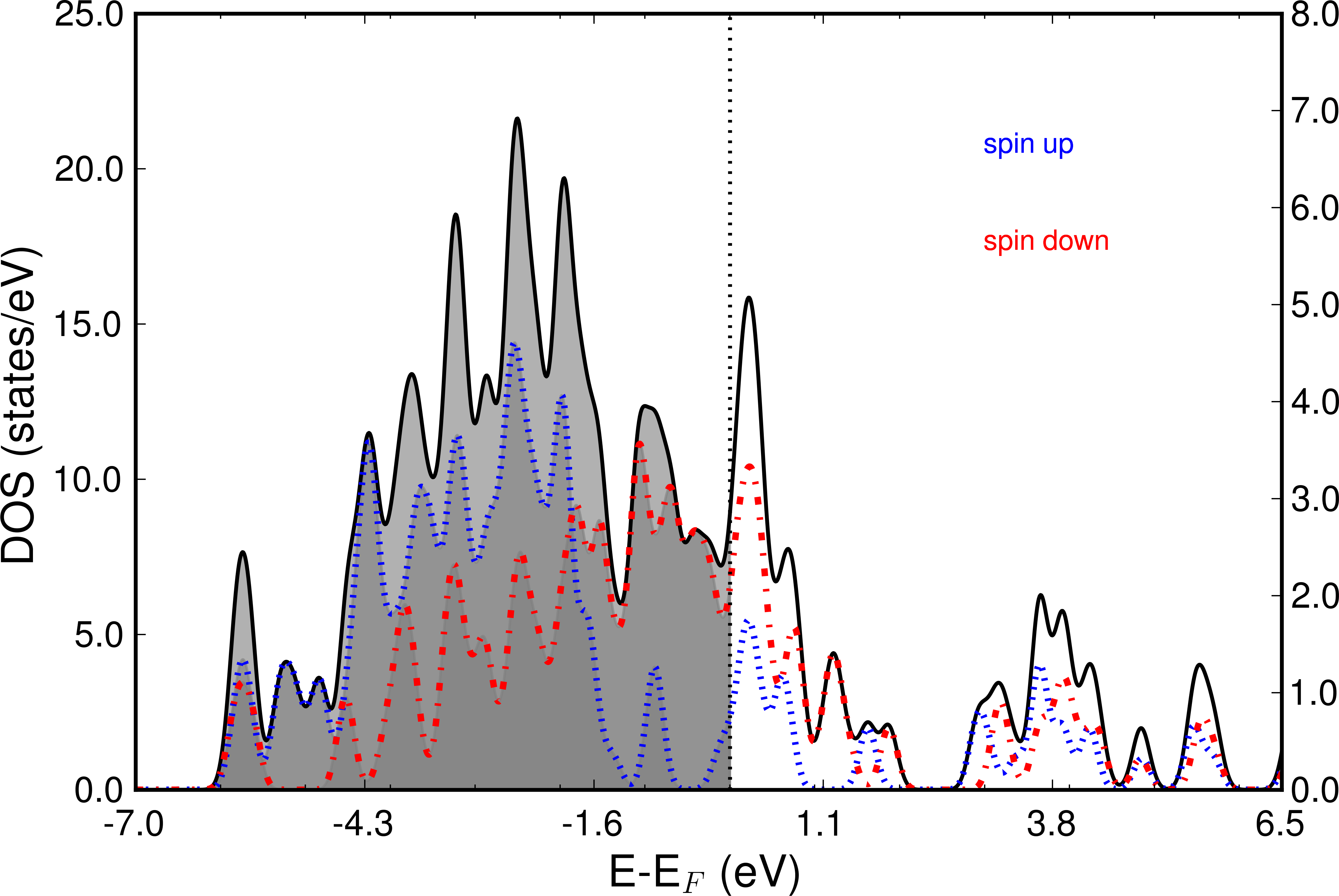
The following image shows the Total DOS and the two spin channels.
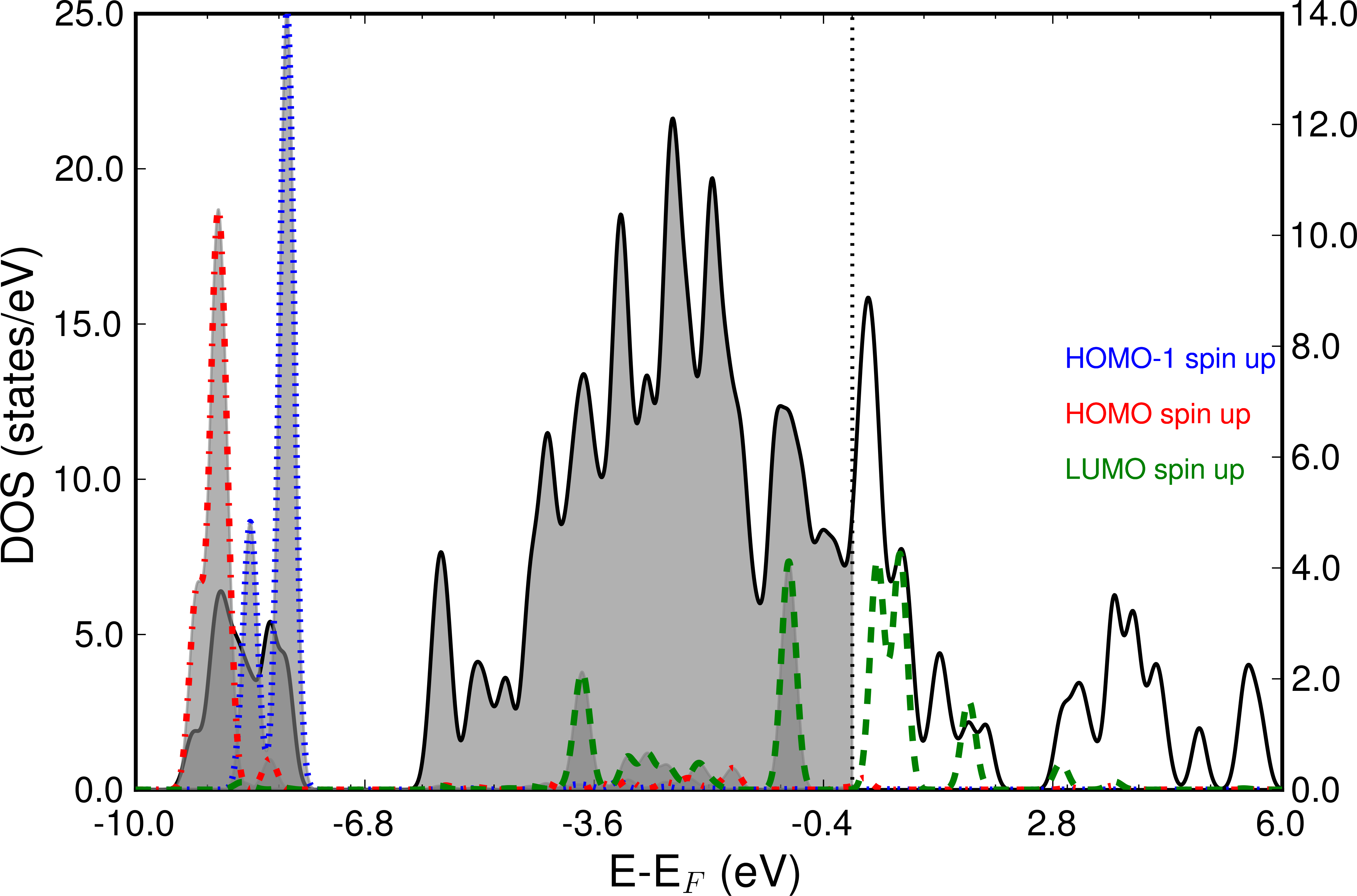
The next picture shows the frontier orbitals of spin channel 1 projected on the total DOS. Especially the LUMO shows strong hybridization with the Nickel d-bands and also is partially occupied. The left scale refers to the total DOS, whereas the right y-scale shows the peak height of the projected MOs.
Example 5: Putting it all together: CO on Cu(100)
For this example we analyze the electronic structure of a CO molecule in a c(2x2) overlayer on Cu(100), before we use this information to calculate the correct electronic transitions.
In the following, the required input files are:
co-on-cu100.param, co-on-cu100.cell, co-on-cu100.deltascf, gasphase.cell, gasphase.param, gasphase.deltascf
co-on-cu100.param
#%BLOCK DEVEL_CODE
#DEVEL_CODE : DeltaSCF
#%ENDBLOCK DEVEL_CODE

#reuse: default
task: SinglePoint

spin_polarized : False
cut_off_energy : 400.0
elec_energy_tol : 1e-07
fix_occupancy : False
iprint : 1
max_scf_cycles : 200
metals_method : dm
mixing_scheme : Pulay
nextra_bands : 50
num_dump_cycles : 0
opt_strategy_bias : 3
smearing_scheme : Gaussian
smearing_width : 0.1
xc_functional : PBE
co-on-cu100.cell
%BLOCK LATTICE_CART
0.0000000000000000 -3.6320000000000001 0.0000000000000000
3.6320000000000001 0.0000000000000000 0.0000000000000000
0.0000000000 0.0000000000 23.614900000
%ENDBLOCK LATTICE_CART

%BLOCK POSITIONS_ABS
Cu      0.02575600      -3.70271100      -7.26400000
Cu      1.84175600      -1.88671100      -7.26400000
Cu      0.02575600      -1.88671100      -5.44800000
Cu      1.84175600      -3.70271100      -5.44800000
Cu      0.02575600      -3.70271100      -3.63200000
Cu      1.84175600      -1.88671100      -3.63200000
Cu      0.02575600      -1.88671100      -1.81600000
Cu      1.84175600      -3.70271100      -1.81600000
Cu      0.02575600      -3.70271100       0.00000000
Cu      1.84175600      -1.88671100       0.00000000
C      0.02575600      -3.70271100       1.90000000
O      0.02575600      -3.70271100       3.00000000
%ENDBLOCK POSITIONS_ABS

FIX_ALL_CELL : True
KPOINTS_MP_GRID : 2 2 1
KPOINTS_MP_OFFSET : 0.25 0.25 0.25
co-on-cu100.deltascf
deltascf_iprint      :  1
deltascf_mode        :  3
deltascf_file        :  gasphase.check
deltascf_constraint  :  5     0.5000  1
deltascf_constraint  :  6     0.5000  2
gasphase.param
#reuse: default
task: SinglePoint

spin_polarized : False
cut_off_energy : 400.0
elec_energy_tol : 1e-07
fix_occupancy : False
iprint : 1
max_scf_cycles : 200
metals_method : dm
mixing_scheme : Pulay
nextra_bands : 50
num_dump_cycles : 0
opt_strategy_bias : 3
smearing_scheme : Gaussian
smearing_width : 0.1
xc_functional : PBE
gasphase.cell
%BLOCK LATTICE_CART
0.0000000000000000 -3.6320000000000001 0.0000000000000000
3.6320000000000001 0.0000000000000000 0.0000000000000000
0.0000000000 0.0000000000 23.614900000
%ENDBLOCK LATTICE_CART

%BLOCK POSITIONS_ABS
C      0.02575600      -3.70271100       1.90000000
O      0.02575600      -3.70271100       3.00000000
%ENDBLOCK POSITIONS_ABS

FIX_ALL_CELL : True
KPOINTS_MP_GRID : 2 2 1
KPOINTS_MP_OFFSET : 0.25 0.25 0.25
gasphase.deltascf
deltascf_mode        :  1
deltascf_iprint      :  1
deltascf_constraint  :   5    0.5000  1    5    5
deltascf_constraint  :   6    0.5000  1    6    6
deltascf_smearing    :  0.01
We start out by calculating the groundstate of the adsorbed molecule and the ground state of the gasphase molecule and by analyzing the MOlPDOS of CO on Cu(100).
- GOOD TO KNOW
- If you ever forget the correct input for <seed>.deltascf or <seed>.molpdos, just run the MolPDOS tool without seed. The printed information is all you need!
TO DO