Example 1: Calculating a friction tensor from FHI-aims data: CO on Cu(100)

In this example we calculate the friction tensor from data previously calculated with FHI-Aims. We do this for CO adsorbed at a top site of a Pd(111) surface. The corresponding friction tensor is a (6x6) matrix.

In order to run this example you need to download the FHI-Aims dataset from following URL and extract it in the example folder

Download Dataset

Code

#    This file is part of coolvib
#
#        coolvib is free software: you can redistribute it and/or modify
#        it under the terms of the GNU General Public License as published by
#        the Free Software Foundation, either version 3 of the License, or
#        (at your option) any later version.
#
#        coolvib is distributed in the hope that it will be useful,
#        but WITHOUT ANY WARRANTY; without even the implied warranty of
#        MERCHANTABILITY or FITNESS FOR A PARTICULAR PURPOSE.  See the
#        GNU General Public License for more details.
#
#        You should have received a copy of the GNU General Public License
#        along with coolvib.  If not, see <http://www.gnu.org/licenses/>.
"""
We calculate the (6x6) friction tensor for 
a CO molecule adsorbed on a Pd(111) top site.
"""

import numpy as np
from ase.io import read
import os, sys
import coolvib
from scipy import linalg as LA
#from ase.visualize import view

#####DEFINE SYSTEM and PARAMETERS######
system = read('CO_on_Pd111/eq/geometry.in')
cell = system
active_atoms = [4,5] # meaning we have two atoms - C - 0 and O - 1
#view(system)

model = coolvib.workflow_tensor(system, code='aims', active_atoms=active_atoms)

finite_difference_incr = 0.0025

keywords = {
    'discretization_type' : 'gaussian',
    'discretization_broadening' : 0.01,
    'discretization_length' : 0.01,
    'max_energy' : 3.00,
    'temperature' : 300,
    'delta_function_type': 'gaussian',
    'delta_function_width': 0.60,
    'perturbing_energy' : 0.0,
    'debug': 0,
        }

print 'workflow initialized and keywords set'

######READ QM INPUT DATA###
model.read_input_data(
        spin=False, 
        path='./CO_on_Pd111/',
        filename='aims.out', 
        active_atoms=active_atoms, 
        incr=finite_difference_incr,
        debug=0,
        )
print 'successfully read QM input data'

############
#We can either calculate the spectral function and evaluate friction 
#from there (discretization commands)

######CALCULATE SPECTRAL FUNCTION###
# model.calculate_spectral_function(mode='default', **keywords)
# # model.read_spectral_function()
# print 'successfully calculated spectral_function'
# model.print_spectral_function('nacs-spectrum.out')
# model.calculate_friction_tensor_from_spectrum(**keywords)
# model.plot_spectral_function()

#######CALCULATE FRICTION TENSOR###

#or we directly calculate friction
model.calculate_friction_tensor( **keywords)

print 'successfully calculated friction tensor'

model.analyse_friction_tensor()
model.print_jmol_friction_eigenvectors()


######project lifetimes along vibrations
hessian_modes = np.loadtxt('CO_on_Pd111/hessian')
for i in range(len(hessian_modes)):
    hessian_modes[i,:]/=np.linalg.norm(hessian_modes[i,:])

from coolvib.constants import time_to_ps
ft= np.dot(hessian_modes,np.dot(model.friction_tensor,hessian_modes.transpose()))/time_to_ps
E, V = np.linalg.eigh(ft)
coolvib.routines.output.print_matrix(ft)

print 'Relaxation rates along vibrational modes in 1/ps'
for i in range(len(ft)):
    print ft[i,i]
print 'Vibrational lifetimes along vibrational modes in 1/ps'
for i in range(len(ft)):
    print 1./ft[i,i]

Detailed Explanation

System Setup

We start by setting up the system using an ASE atoms object and we initialize our workflow_tensor class with

import coolvib
model = coolvib.workflow_tensor(system, code='aims', active_atoms=[4,5])

, where active_atoms specifies the indices of the atoms we want to include in the calculation of the friction tensor. Model is an instance of the coolvib.convenience.workflow_tensor.workflow_tensor class that guides us through the calculation and bundles all data and functions.

Reading input data

After defining all keywords we can read the FHI-Aims data by using coolvib.convenience.workflow_tensor.workflow_tensor.read_input_data().

The parser assumes that the input data is given as a set of directories with eq refering to the calculation at equilibrium position and a3c0+ or a3c0- refering to displacements in positive and negative directions for atom3 and the cartesian x component (c0 = x, c1 = y, c2 = z).

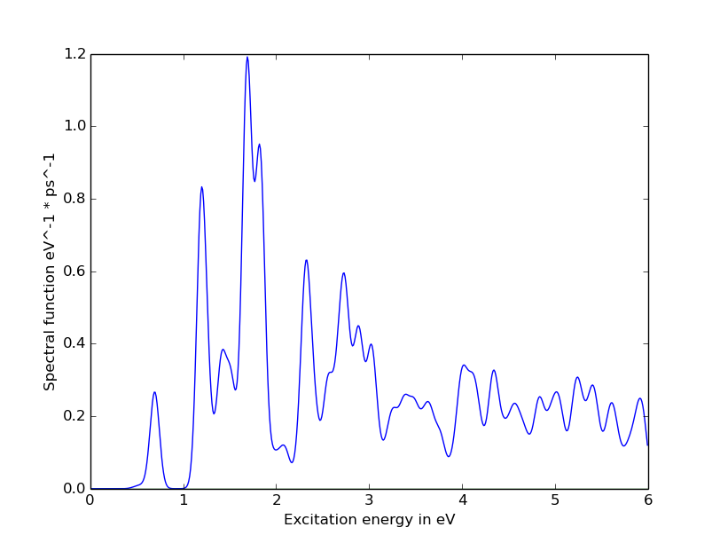
Calculating the spectral function

This is an optional step when calculating the friction tensor and at the moment only serves analysis purposes.

Using coolvib.convenience.workflow_tensor.workflow_tensor.calculate_spectral_function() we can calculate the spectral functions along all cartesian components and all combinations of cartesian components. This includes loops over all possible excitations and construction of the electron-phonon spectral function on a discrete grid. This discretization is determined by following keywords:

discretization_type

Specifies which broadening function is used to discretize the individual excitations, for more details see coolvib.routines.discretize_peak()

discretization_broadening

Specifies the width that is used to generate a finite width discrete representation of the peak and intensity (in eV)

discretization_length

Specifies the bin width of equidistant grid on which the spectral function is represented (in eV).

max_energy

Specifies the maximum extend beyond the fermi level for which the spectral function is calculated. The default is 3 eV. A safe value is 5 times the delta_function_width+perturbing_energy

The calculated spectral functions can be printed to file using coolvib.convenience.workflow_tensor.workflow_tensor.print_spectral_function(). This file can be post-processed and further analyzed using scripts from coolvib.tools.

Calculating the friction tensor and analysis

In order to finally arrive at the friction tensor one either has to integrate the spectral functions over a delta function (see coolvib.routines.evaluate_delta_function()). This is where the main approximations of the underlying method are applied. The width, position and shape of the delta function are controlled by following keywords:

delta_function_type

Specifies the type of delta function representation to be used

delta_function_width

Specifies the width of the delta function representation (in eV)

perturbing_energy

Specifies the position of the delta function representation. Typically this is chosen to be at the Fermi level under the quasi-static approximation (see Theory)

Convergence with respect to the decay rates and lifetimes has to be validated for the above parameters.

The function coolvib.convenience.workflow_tensor.workflow_tensor.calculate_friction_tensor_from_spectrum() performs this integration and sets up the tensor.

One can directly calculate the friction tensor by using coolvib.convenience.workflow_tensor.calculate_friction_tensor(), as it is done in this example

Analysis and printing of the tensor, its eigenvalues and eigenfunctions as well as the inverse of the eigenvalues (the principal lifetimes) can be done using coolvib.convenience.workflow_tensor.workflow_tensor.analyse_friction_tensor().

Results

The expected results are

Friction Tensor

0 1 2 3 4 5

0 3.2947e-01 -5.1951e-05 -1.4243e-04 -9.7699e-02 2.4844e-05 -1.1275e-04 1 -5.1951e-05 3.2955e-01 -1.4646e-04 1.2838e-05 -9.7716e-02 -1.1241e-04 2 -1.4243e-04 -1.4646e-04 1.6286e-01 4.2497e-05 4.2755e-05 -1.1424e-02 3 -9.7699e-02 1.2838e-05 4.2497e-05 2.9649e-02 -5.7152e-06 2.9358e-05 4 2.4844e-05 -9.7716e-02 4.2755e-05 -5.7152e-06 2.9654e-02 3.0400e-05 5 -1.1275e-04 -1.1241e-04 -1.1424e-02 2.9358e-05 3.0400e-05 6.7262e-03

Friction Eigenvalues in 1/ps

0 1 2 3 4 5

0.0006 0.0006 0.0059 0.1637 0.3585 0.3586

Friction Eigenvectors

0 1 2 3 4 5

0 -2.7421e-01 -7.6918e-02 -1.3190e-04 6.8885e-04 -8.5161e-01 4.4006e-01 1 7.6930e-02 -2.7419e-01 -1.8838e-04 7.0623e-04 -4.4007e-01 -8.5161e-01 2 -3.7931e-05 -5.5541e-05 -7.2589e-02 9.9736e-01 1.0090e-03 3.3623e-04 3 -9.2294e-01 -2.5899e-01 8.2028e-04 -2.0170e-04 2.5301e-01 -1.3073e-01 4 2.5899e-01 -9.2295e-01 6.3231e-04 -2.1305e-04 1.3071e-01 2.5300e-01 5 -5.7038e-04 -7.3214e-04 -9.9736e-01 -7.2590e-02 4.1327e-04 1.3106e-04

Principal lifetimes in ps

0 1 2 3 4 5

1605.4274 1597.3460 169.6452 6.1092 2.7896 2.7885