# nbi:hide_in
import nbinteract as nbi
import numpy as np
import scipy as sp
The particle in a box in 1D
Here's a quick reminder of the particle in a box
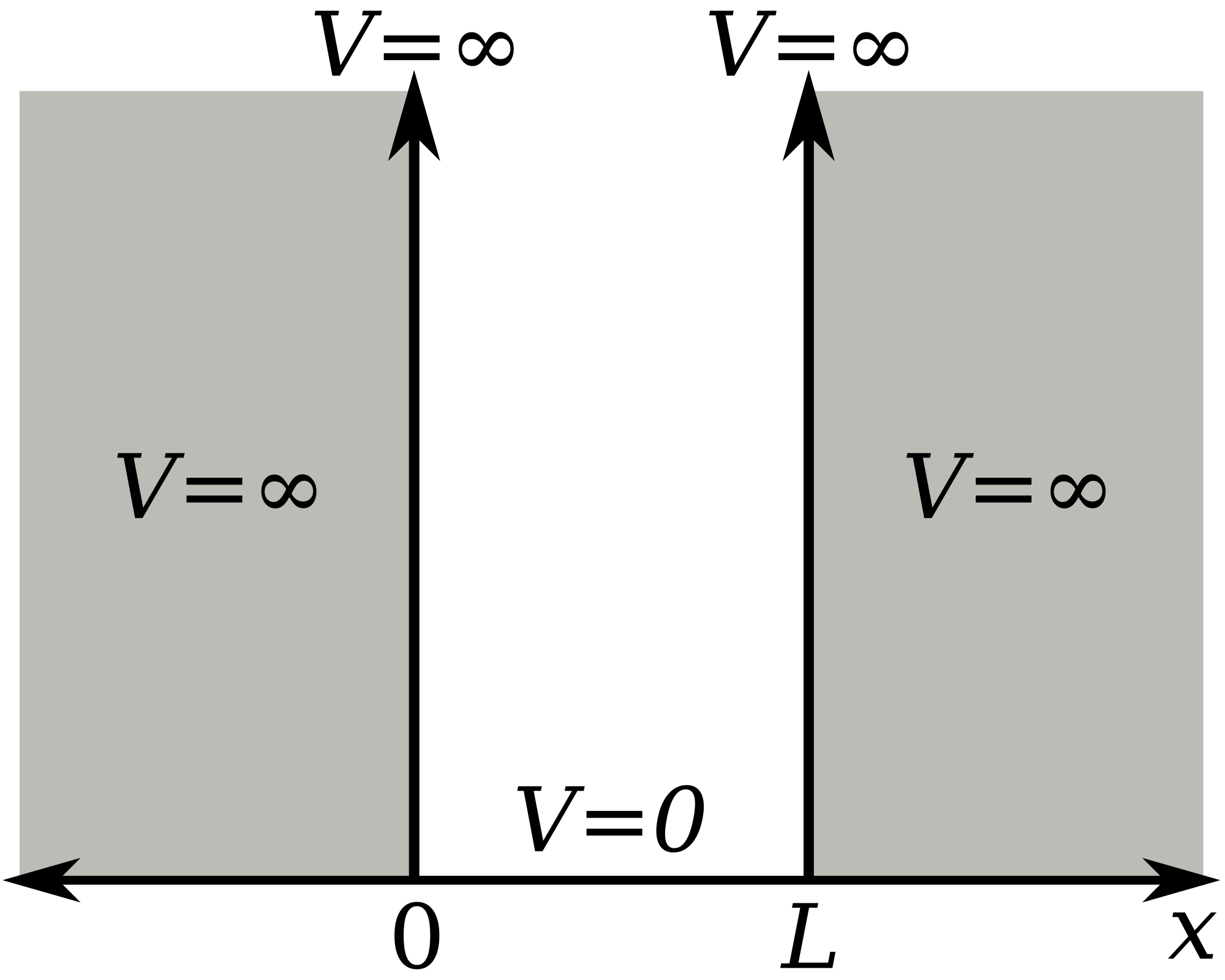
Schrödinger equation (SE): $\hat{H}\psi = E\psi $
SE: action of energy operator $\hat{H}$ defines the energy and wave function $\psi$
$$ \hat{H} = -\frac{\hbar^2}{2m}\frac{d^2}{dx^2} +V $$
boundary conditions: $ \psi(0) = 0 \quad\text{and}\quad \psi(L) = 0 $
wave function
$$ \psi_n(x) = \sqrt{\frac{2}{L}}\sin{\frac{n\pi x}{L}} $$
energies
$$ E_n = \frac{\hbar^2\pi^2}{2m}\frac{n^2}{L^2} $$
# nbi:hide_in
def make_xgrid(start, stop, N):
    x = np.linspace(start,stop,N)
    return x
# nbi:hide_in
def potential(x, box_l=0.0, box_r=5.0, height=100000.0):
    pot = np.zeros_like(x)     #isn't numpy great? This generates an array with zeros, which has the same shape like x

    for i, xvalue in enumerate(x): #we loop through all x values
        #enumerate is really nice.
        #It allows us to loop through an array and, for each value, gives us an index i and the actual xvalue
        if (xvalue<box_l): #left wall
            pot[i] = height
        elif (xvalue> box_l and xvalue < box_r): #inside the box
            pot[i] = 0.0
        elif (xvalue>box_r): #right wall
            pot[i] = height
        else:

            raise ValueError("COMPUTER SAYS NO. This point should never be reached.")
    return pot
# nbi:hide_in
def create_H(x, pot):
    hbar = 1
    m = 1
    dx = x[1]-x[0]

    import scipy.ndimage
    L = scipy.ndimage.laplace(np.eye(len(x)), mode='wrap')/(2.0*dx*dx) #np.eye is a diagonal unit matrix (I) with size 'x' by 'x'
    T= -(1./2.)*((hbar**2)/m)*L

    V = np.diag(pot)   #np.diag takes a list of numbers and puts it onto the diagonal; the offdiagonals are 0

    H = T+V
    return H
# nbi:hide_in
def diagonalise_H(H):
    import scipy.linalg as la
    E, psi = la.eigh(H)
    return E, psi
# nbi:hide_in

#### %matplotlib notebook
%matplotlib inline
import matplotlib.pyplot as plt
from ipywidgets import interact, interactive, fixed, interact_manual

def plot_pib1d(x, pot, E, psi, n=0):
        """
        plots the energies, the wave function and the probability density with interactive handles.
        """

        n=n-1
        import matplotlib.gridspec as gridspec
        plt.figure(figsize=(11, 8), dpi= 80, facecolor='w', edgecolor='k') # figsize determines the actual size of the figure
        gs1 = gridspec.GridSpec(2, 3)
        gs1.update(left=0.05, right=0.90, wspace=0.35,hspace=0.25)
        ax1 = plt.subplot(gs1[: ,0])
        ax2 = plt.subplot(gs1[0, 1:])
        ax3 = plt.subplot(gs1[1, 1:])


        ax1.plot(x, pot, color='gray')
        ax1.plot(np.ones(len(E)), E, lw=0.0, marker='_',ms=4000, color='blue')
        ax1.plot(1, E[n], lw=0.0, marker='_',ms=4000, color='red')
        ax1.set_ylim(-1,21)
        ax2.plot(x, psi[:,n])
        ax3.plot(x, psi[:,n]*psi[:,n])

        #figure out boundaries
        start=0; stop=0
        for i, p in enumerate(pot):
            if (p>-0.001 and p<0.001):
                start=x[i-1]
                break
        for i, p in enumerate(pot):
            if (p>-0.001 and p<0.001):
                stop=x[i+1]

        ax2.axvline(start, color='gray')
        ax2.axvline(stop, color='gray')
        ax3.axvline(start, color='gray')
        ax3.axvline(stop, color='gray')
        ax3.axhline(0.0,color='gray')

        #Labeling of x and y axes
        ax1.set_xlabel('x',fontsize=14)
        ax1.set_ylabel('Energy [eV]',fontsize=14)
        ax2.set_ylabel(r'wave function $\psi(x)$',fontsize=14)
        ax3.set_ylabel(r'density $|\psi|^2$(x)',fontsize=14)
        ax2.set_xlabel(r'x',fontsize=14)
        ax3.set_xlabel(r'x',fontsize=14)

        #Show the final result
        plt.show()
        return plot_pib1d
# nbi:hide_in
def pib1d(N=100, box_l=0.0, box_r=5.0, height=100000.0, n=0):
    """
    calculates and visualises the energies and wave functions of the 1d particle in a box

    This program takes the number of grid points and the start and end point of the box as arguments and
    returns a visualisation.
    """

    #make an x axis
    x = make_xgrid(box_l-1.0,box_r+1.0,N)
    #create a box potential on that axis
    pot = potential(x,box_l, box_r, height)
    #calculate Hamiltonian
    H = create_H(x,pot)
    #diagonalise Hamiltonian, solve for E and psi
    E, psi = diagonalise_H(H)
    plot_pib1d(x, pot, E, psi, n)

    #If the function doesn't have a return value and simply executes a number of commands,
    #we simply return the logical value true when everything ran smoothly to the end
    return pib1d
# nbi:hide_in
#plot results
N = 100
box_l = 0.0
box_r = 5.0
height = 100000.0
#pib1d(N,box_l,box_r, height)
interact(pib1d, N=fixed(N), box_l=fixed(box_l), box_r=(1.0,10.0), height=(0.,10000,10), n=range(1,21))
The particle in a slanted box
# nbi:hide_in

#potential function
def tilted_potential(x, box_l=0.0, box_r=5.0, height=100000.0, grad=1.0):
    pot = np.zeros_like(x)     #isn't numpy great? This generates an array with zeros, which has the same shape like x

    for i, xvalue in enumerate(x): #we loop through all x values
        #enumerate is really nice.
        #It allows us to loop through an array and, for each value, gives us an index i and the actual xvalue
        if (xvalue<box_l): #left wall
            pot[i] = height
        elif (xvalue> box_l and xvalue < box_r): #inside the box
            pot[i] = xvalue*grad
        elif (xvalue>box_r): #right wall
            pot[i] = height
        else:
            raise ValueError("COMPUTER SAYS NO. This point should never be reached.")
    return pot


#new main program where we replaced the potential
def tilted_pib(N,box_l=0.0,box_r=5.0, height=10000.0,n=1, grad=1.0):

    x = make_xgrid(box_l-1.0,box_r+1.0,N)
    ######ONLY THE FOLLOWING LINES ARE DIFFERENT
    x0 = (box_l+box_r)/2  #define the centre of the harmonic oscillator in the middle of the box
    pot = tilted_potential(x, box_l, box_r, height, grad)
    ######END OF DIFFERENCE##########
    H = create_H(x,pot)
    E, psi = diagonalise_H(H)
    plot_pib1d(x, pot, E, psi, n)

    return tilted_pib
# nbi:hide_in
#plot results
N = 100
box_l = 0.0
box_r = 5.0
height = 100000.0
#pib1d(N,box_l,box_r, height)
interact(tilted_pib, N=fixed(N), box_l=fixed(box_l), box_r=fixed(box_r), height=fixed(height), n=range(1,20), grad=(0.,10.))
The Harmonic oscillator
# nbi:hide_in

#potential function
def harmonic_potential(x, x0=2.5, k=10.):
    """
    Function calculates harmonic potential on x-axis centred around x0 with spring constant k
    """
    return 0.5*k*(x-x0)*(x-x0)


#new main program where we replaced the potential
def HO1D(N,box_l,box_r, k=10.0, n=0):

    x = make_xgrid(box_l-1.0,box_r+1.0,N)
    ######ONLY THE FOLLOWING LINES ARE DIFFERENT
    x0 = (box_l+box_r)/2  #define the centre of the harmonic oscillator in the middle of the box
    pot = harmonic_potential(x, x0, k)
    ######END OF DIFFERENCE##########
    H = create_H(x,pot)
    E, psi = diagonalise_H(H)
    plot_pib1d(x, pot, E, psi, n)

    return HO1D
# nbi:hide_in
#Number of grid points
N = 100
box_l = 0.0
box_r = 5.0
height = 10.0
interact(HO1D, N=fixed(N),box_l=fixed(box_l),box_r = fixed(box_r),k=(1.,100.), n=range(1,20))